This is part 4 and the final post of this JSON series. We are going to play with Smartsheet data because its adds to our examples of varying JSON structure. Note that Power BI already has a connector for Smartsheet. There is also a Python SDK for Smartsheet, but we are going to use the Python requests library so that we can start from scratch and learn how to navigate the JSON structure.
We will follow the same approach as the previous post i.e. focus on understanding the structure, draw from our existing patterns and add one or two new techniques to our arsenal.
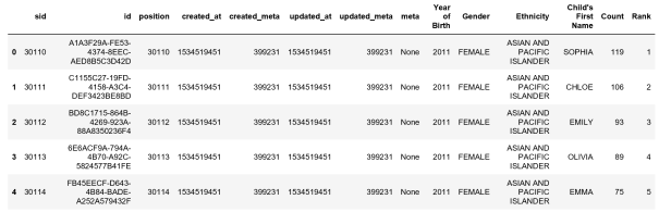
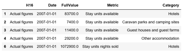
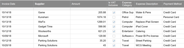
Below is the screenshot of the actual Smartsheet we will be working with.
Accessing the Smartsheet API
API access is available during the free trial period. If you want to play, have a look at how to generate the token so that you can authenticate your API access. If you have been following my posts, you would know by now that I store my secure information (such as API tokens) in the user environment variables on by development computer.
To access the API we need to create the endpoint from the Smartsheet API URL and the sheet ID for the sheet you want to access. We also need the token which we pass to the request header. The code to do this is as follows:
import json

auth = os.getenv('SMARTSHEET_TOKEN')
smartsheet = 'https://api.smartsheet.com/2.0/sheets/'
sheetid = '3220009594972036'
uri = smartsheet + sheetid
header = {'Authorization': "Bearer " + auth,
          'Content-Type': 'application/json'}

req = requests.get(uri, headers=header)
data = json.loads(req.text)
In the above script, the last line converts the request text into a Python dictionary structure.
Understanding the data structures
This is the critical step. Understand the problem … and in this case it means read the Smartsheet documentation and compare it to the physical structure. This time round we are going to use the pretty print (pprint) library for the latter.
import pprint
pprint.pprint(data)
The documentation tells us that there is a sheet which is the main object. The sheet contains the columns (metadata) object, a rows object and cells object. It also tells us that a collection of cells form a row. When we explore the physical structure we see that this is indeed the case.


So the column metadata and rows are referenced directly from the sheet object, and the cells are referenced from the row object. We could thus access the columns and rows dictionaries directly.
pprint.pprint(data['columns'])
pprint.pprint(data['rows'])
Building the dataframe
The process we are going to follow is to create an empty dataframe from the column metadata (using the ‘title’ key: value pair). We are then going to iterate over the rows and cells and append the values to the new dataframe.
We are firstly going to create a list of columns. This has a dual purpose. We will use it to create the empty dataframe, then we will re-use it to create row dictionaries that we will append to the dataframe.
cols = []
for col in data['columns']:
    cols.append(col['title'])

Creating the empty dataframe from this is straightforward.
import pandas
df = pandas.DataFrame(columns=cols)
To append the rows, we iterate over the rows with a loop and we use a nested loop to iterate over the cells. The cells in each row are added to a list, but first we trap empty values in the VAT field.
for row in data['rows']:
values = [] #re-initialise the values list for each row
for cell in row['cells']:
if cell.get('value'): #handle the empty values
values.append( cell['value'])
else:
values.append('')
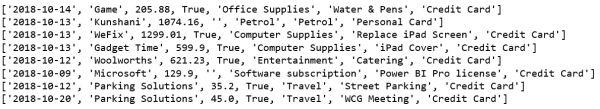
print(values)
Now we need a new trick to added these lists to the dataframe. We are going to use a function called zip. Zip must be used in conjunction with an iterator such as a list or dictionary.

We are going to use this to combine our columns and rows into a dictionary that we append to the dataframe. The complete script is below.
import json, pandas

auth = os.getenv('SMARTSHEET_TOKEN')
smartsheet = 'https://api.smartsheet.com/2.0/sheets/'
sheetid = '3220009594972036'
uri = smartsheet + sheetid
header = {'Authorization': "Bearer " + auth,
          'Content-Type': 'application/json'}

req = requests.get(uri, headers=header)
data = json.loads(req.text)

cols = []
for col in data['columns']:
    cols.append(col['title'])

df = pandas.DataFrame(columns=cols)

for row in data['rows']:
    values = [] #re-initilise the values list for each row
    for cell in row['cells']:
        if cell.get('value'): #handle the empty values
            values.append( cell['value'])
        else:
            values.append('')
    df = df.append(dict(zip(cols, values)), ignore_index=True)

The moral of the story
While JSON provides a great data interchange standard, implementation of the file format will vary. This means we will always need to make sure we understand the structure and select the required techniques to create an analysis ready format.
This post concludes the JSON series, but will revisit the topic when new scenarios pop up.